23.7.1. Orbital Mobility

This mobility model was originally developed by Tim Schubert as part of ns-3-leo [4]. It was then ported, refactored and optimized by Thiago Myazaki as part of Google Summer of Code (GSoC) 2025.

It allows for the configuration of satellite scenarios, with the objective to create an example integrating LEO satellites using beamforming, channel and propagation models from the NR Module and ns-3, leveraging a helper model to aid the instantiation of LEO satellites.

It models simple circular orbits with constant orbital velocity.

In addition to the mobility model, we have also ported an example from ns-3-leo [4] that outputs position traces as ECEF coordinates. Using a Python script developed during the project, plot-orbital-traces.py, we produced animated plots that helped validate the nodes’ initial positions and their movement over time, under different configurations of numbers of nodes, inclination, and altitude.

We also have a unified example (leo-satellite-example.cc) that combines three use cases into a single program controlled by the --mode switch: orbit for mobility tracing, antenna for antenna pointing toward a ground station, and channel for full 3GPP NTN propagation loss estimation.

23.7.1.1. Characteristics & Assumptions

The LEO mobility model relies on classical two-body orbital mechanics. The following references provide the theoretical background:

• Orbital mechanics — general overview of orbital mechanics and the two-body problem.

• Orbital elements — parameters defining an orbit (semi-major axis, eccentricity, inclination, RAAN, argument of perigee, true anomaly).

• Kepler’s laws of planetary motion — the third law is used to derive the orbital angular velocity from the satellite altitude.

• Low Earth orbit — definition and typical characteristics of LEO.

The model has the following assumptions:

• Orbit type: only models ideal circular orbits. There is no support for elliptical orbits.

• Fixed speed: Since the orbit is circular and not elliptical, we assume the satellite nodes are moving at constant speed along their orbits, given a certain altitude.

• Static Earth: While the model takes into consideration Earth’s rotation, it does not consider Earth’s orbit around the sun; i.e., the Earth is static.

• In the plots, Earth is modeled as a perfect sphere.

The model computes satellite positions in three steps:

• First step: Compute the satellite’s angular position along its orbit from the initial orbital offset and the angular velocity (derived from altitude via Keplerian mechanics, see Orbital elements) multiplied by the elapsed simulation time.

• Second step: Apply orbital plane inclination relative to the equator and rotation by the RAAN.

• Third step: Apply the Rodrigues rotation formula (see Rodrigues’ rotation formula) to rotate the satellite around the orbital plane normal by the computed angular position.

The figures below illustrate how satellites are distributed along their orbits at different angular spacings. They can be plotted with the help of the plot-orbital-traces.py script.

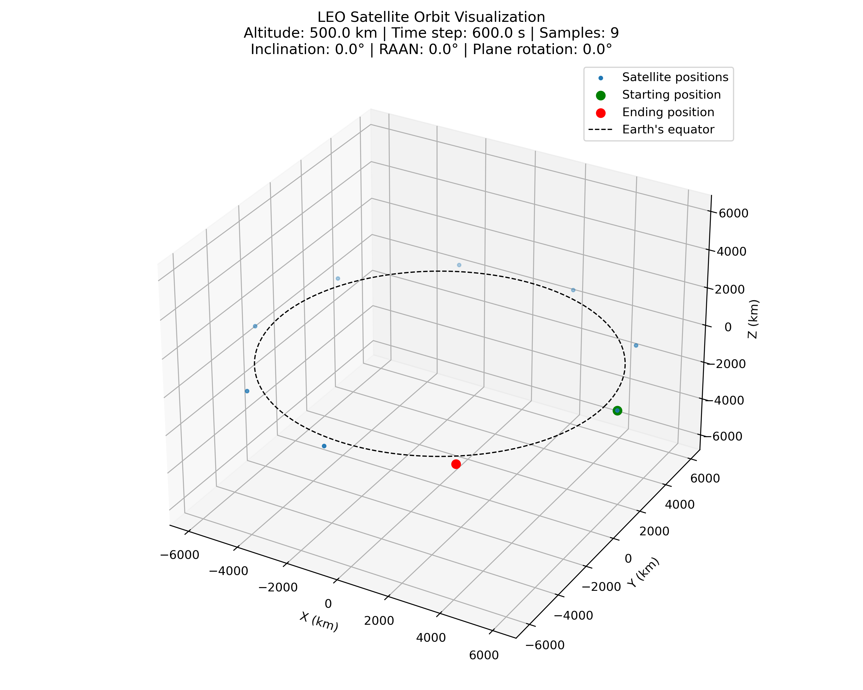
Fig. 23.1 LEO orbit with 600 s resolution, settable via the LeoCircularOrbitMobilityModel::Resolution attribute

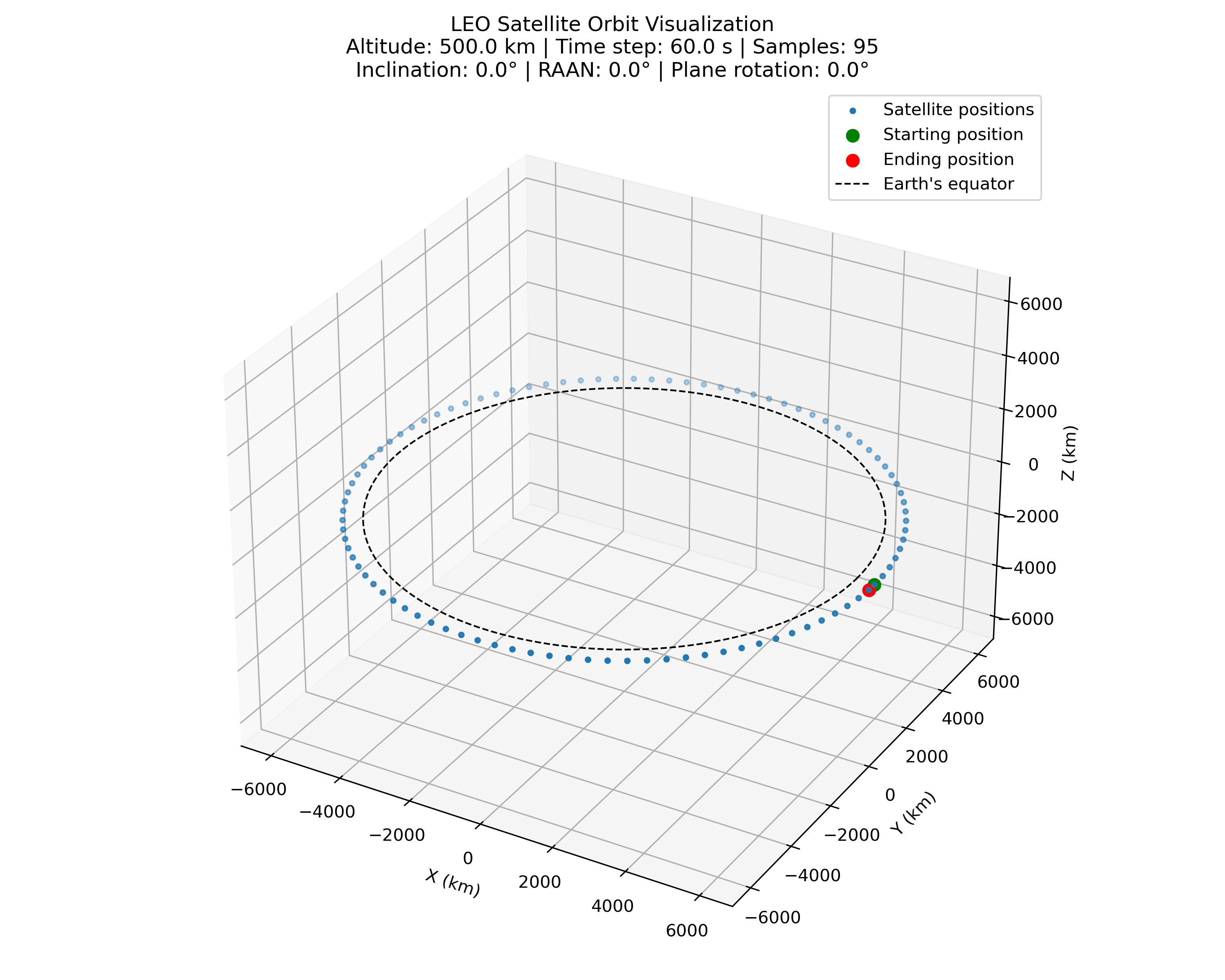
Fig. 23.2 LEO orbit with 60 s resolution

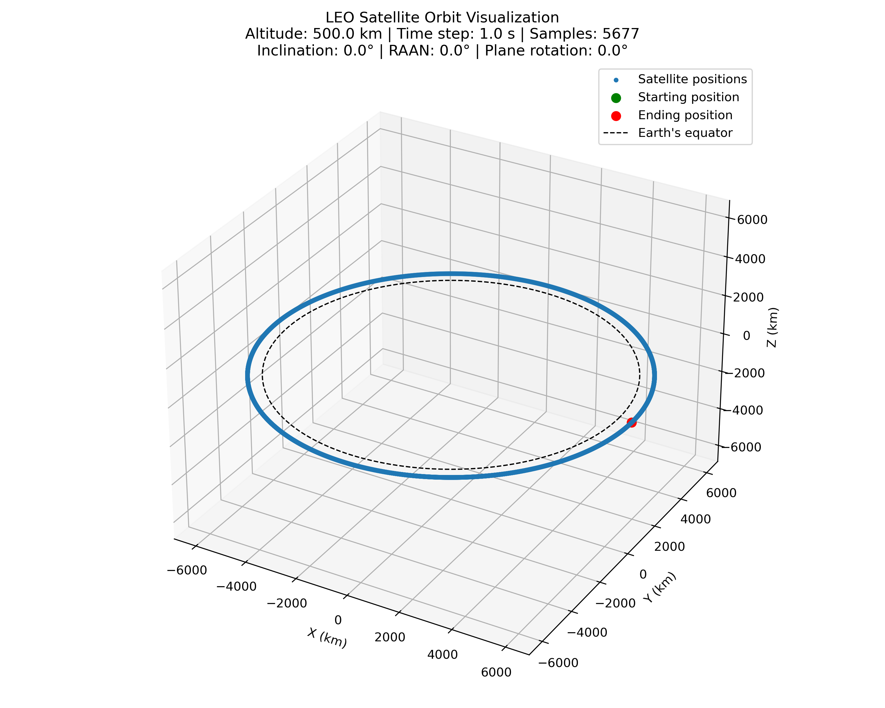
Fig. 23.3 LEO orbit with 1 s resolution

These examples illustrate the trade-off between the resolution time step and the path accuracy. With a coarser resolution (Fig. 23.1), the satellite’s movement appears as larger discrete jumps, while a finer resolution (Fig. 23.3) provides a smoother and more precise representation of the orbital trajectory at the cost of more frequent mobility updates. The intermediate case (Fig. 23.2) shows the effect of a 60 s resolution.

After precomputing these, we apply the plane inclination with respect to the equator, as shown in Fig. 23.4, where we add a 30 degree inclination to the orbital plane with respect to the equator.

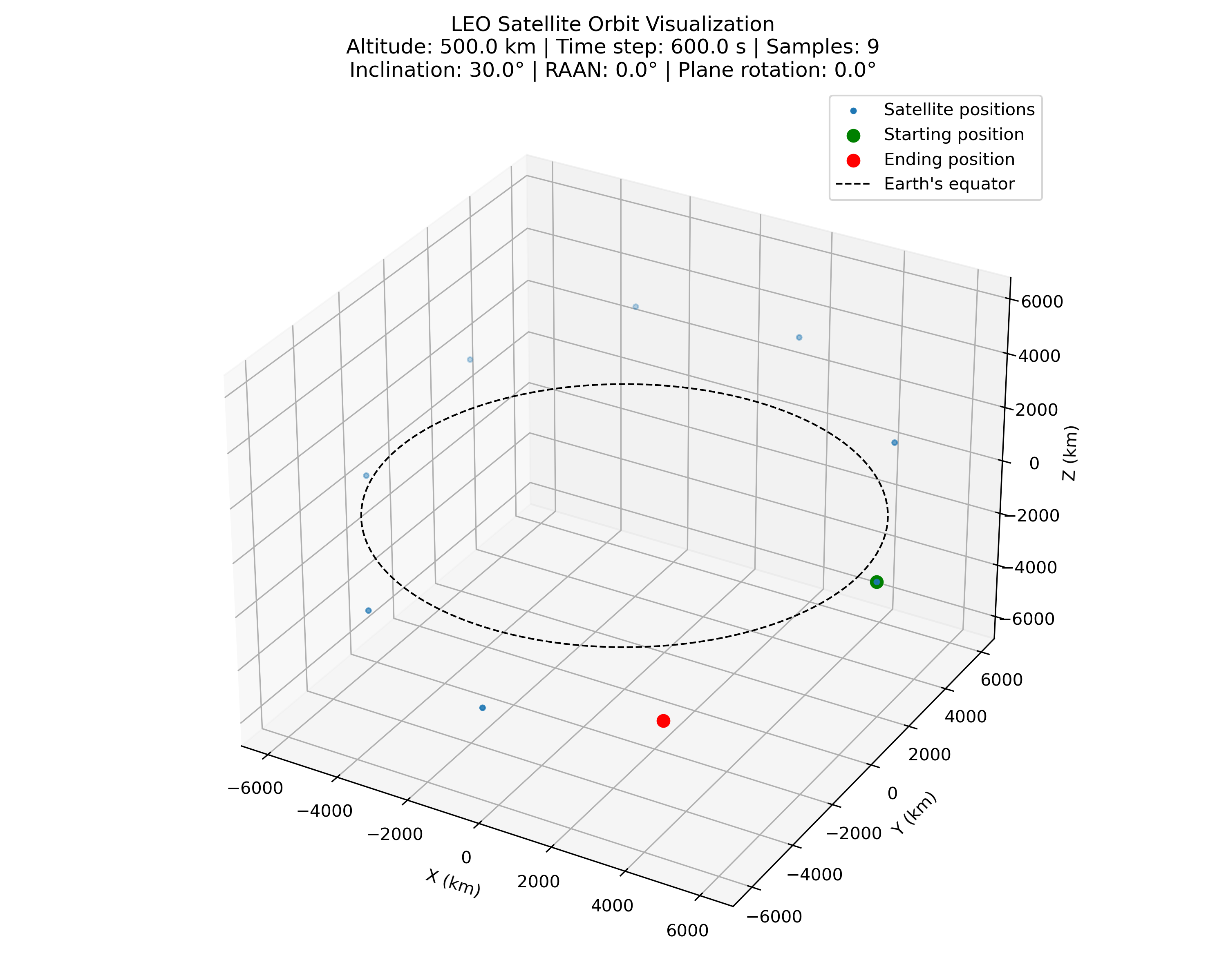
Fig. 23.4 LEO orbit with 30 degrees of inclination, settable via the LeoCircularOrbitMobilityModel::Inclination attribute

When we have multiple orbital planes per constellation, we divide 360 degrees by the number of planes, and apply a Z-axis rotation relative to the RAAN, starting from the prime meridian. This step effectively spaces the orbital planes out around the constellation.

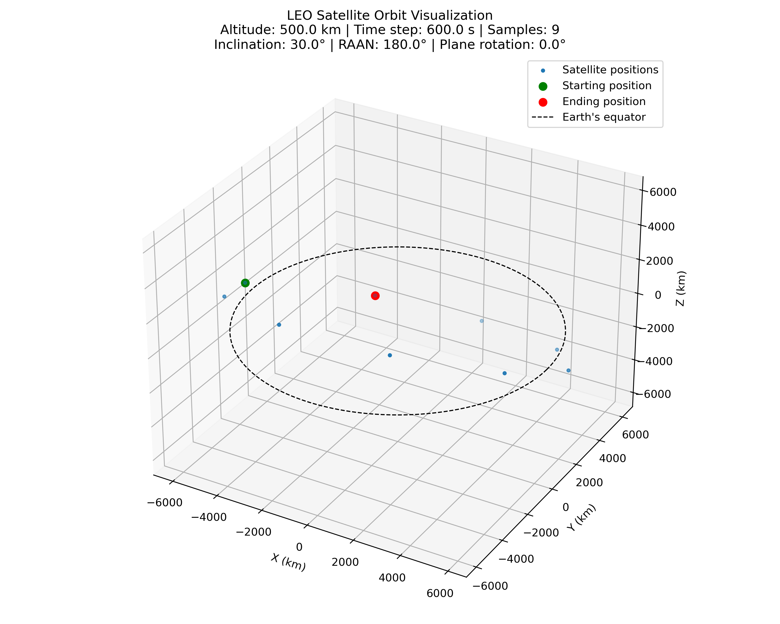
Fig. 23.5 LEO orbit with 30 degrees of inclination and 180 degrees of RAAN rotation

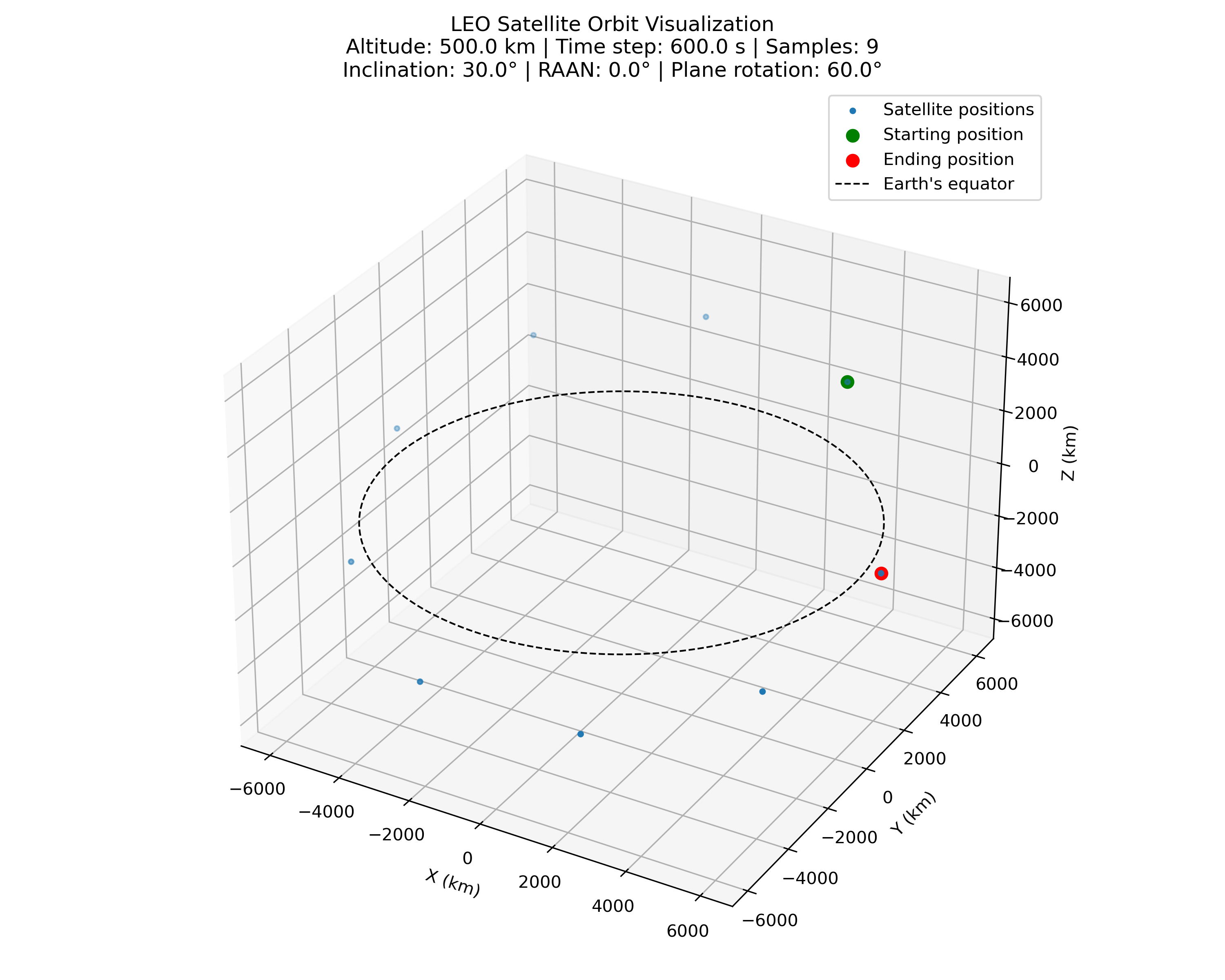
Fig. 23.6 LEO orbit with 30 degrees of inclination, 0 degrees of RAAN rotation, and 60 degrees of plane rotation

For example, with two orbital planes, we would have them separated by 180 degrees, as shown in Fig. 23.4 and Fig. 23.5.

The third and final step is to apply a rotation around the orbital plane normal vector, like adjusting a volume dial, to emulate the orbital movement of the satellite in its orbit. For example, compare Fig. 23.4 and Fig. 23.6.

23.7.1.2. Usage

There are three approaches to setting up a LEO satellite constellation:

• Approach 1: Use a CSV file with constellation parameters, leveraging the LeoOrbitNodeHelper to create satellite nodes and install orbital mobility in a single step.

• Approach 2: Use LeoOrbitalShell objects with the LeoOrbitNodeHelper to configure constellations programmatically and install orbital mobility in a single step.

• Approach 3: Use the standard ns-3 MobilityHelper and PositionAllocator pattern directly, which allows for more fine-grained control over node creation and mobility.

Users will typically want to use the first two approaches.

Approach 1: CSV file with constellation parameters

A CSV file can define one or more orbital shells, each with different altitude, inclination, number of planes, and number of satellites per plane. For example, a file representing part of the Starlink constellation (examples/leo/starlink.csv):

# altitudeKm,inclinationDegrees,numberOfPlanes,numberOfSatellitesPerPlane
1150.0,53.0,32,50
1110.0,53.8,32,50
1130.0,74.0,8,50
(...)

The helper reads the file, creates the appropriate number of nodes for all shells, and installs orbital mobility on each:

std::string orbitFile("examples/leo/starlink.csv");
LeoOrbitNodeHelper orbit(resolution);
NodeContainer satellites = orbit.CreateNodesAndInstallMobility(orbitFile);

The resolution parameter is a Time value that controls how frequently the mobility model fires CourseChange trace notifications. It does not affect the accuracy of the orbital position model itself; satellite positions are always computed exactly on demand when GetPosition() is called. The resolution is handled separately from the orbital parameters (altitude, inclination, planes, satellites) because it is not a property of the orbit but rather a simulation-level control over how often trace callbacks are invoked.

Approach 2: LeoOrbitalShell objects

The LeoOrbitalShell class bundles the following orbital parameters:

• Altitude in kilometers

• Inclination angle in degrees

• Number of planes

• Number of satellites per plane

• Optional Walker Delta phasing factor

• Optional RAAN span in degrees (for Walker Star constellations)

One or more LeoOrbitalShell objects can be passed directly to the helper:

LeoOrbitNodeHelper orbit(resolution);

// Single shell
NodeContainer satellites = orbit.CreateNodesAndInstallMobility(LeoOrbitalShell(1200, 30, 1, 2));

// Multiple shells
NodeContainer satellites = orbit.CreateNodesAndInstallMobility(
    {LeoOrbitalShell(1200, 30, 32, 16), LeoOrbitalShell(1180, 45, 12, 10)});

// Walker Delta 53: 1600/32/1 constellation with phasing factor F = 1
NodeContainer satellites = orbit.CreateNodesAndInstallMobility(LeoOrbitalShell(1200, 53, 32, 50, 1));

Walker Delta constellations are specified in the literature using the notation i: T/P/F, where i is the inclination in degrees, T is the total number of satellites, P is the number of equally spaced orbital planes, and F is the phasing factor. The LeoOrbitalShell constructor takes the number of satellites per plane S rather than the total (with T = P * S); the optional fifth parameter sets the phasing factor F. F staggers satellites in adjacent planes by F * 360 / T degrees. Without phasing (F = 0, the default), all planes have their first satellite at the same orbital offset.

For Walker Star constellations (e.g., Iridium), orbital planes are distributed over 180 degrees instead of 360 degrees. Set the raanSpanDeg member on the LeoOrbitalShell object:

// Walker Star: Iridium-like 86.4: 66/6/1 constellation
LeoOrbitalShell orbit(780, 86.4, 6, 11, 1);
orbit.raanSpanDeg = 180.0;
NodeContainer satellites = helper.CreateNodesAndInstallMobility(orbit);

The RaanSpanDeg attribute on LeoCircularOrbitPositionAllocator can also be set directly when using approach 3.

In both approaches 1 and 2, CreateNodesAndInstallMobility() returns a NodeContainer with all satellite nodes already placed at their initial orbital positions.

Approach 3: Standard MobilityHelper pattern

For a single orbital shell, the standard ns-3 MobilityHelper and PositionAllocator pattern can be used directly:

uint16_t numOrbits = 1;
int32_t numSatellites = 16;
NodeContainer satellites(numOrbits * numSatellites);

MobilityHelper mobility;
mobility.SetPositionAllocator("ns3::LeoCircularOrbitPositionAllocator",
                              "NumOrbits", IntegerValue(numOrbits),
                              "NumSatellites", IntegerValue(numSatellites));
mobility.SetMobilityModel("ns3::LeoCircularOrbitMobilityModel",
                          "Altitude", DoubleValue(1200),
                          "Inclination", DoubleValue(30));
mobility.Install(satellites);

When using this approach, note the following caveats:

• The number of nodes in the NodeContainer must equal NumOrbits * NumSatellites. If these are inconsistent, the position allocator will wrap around or leave nodes at default positions.

• The Altitude and Inclination attributes on the mobility model apply uniformly to all nodes in a single Install() call. For multi-shell constellations (e.g., Starlink with shells at different altitudes), a separate MobilityHelper and Install() call is required for each shell.

23.7.1.3. Resolution

As described above, the Resolution attribute controls how often CourseChange trace notifications are fired. A value of zero disables periodic notifications entirely.

23.7.1.4. leo-satellite-example

This unified example combines three use cases into a single program, controlled by the --mode switch. It sets up a LEO constellation (from a CSV file or a default orbit), places a ground station, and optionally steers each satellite’s antenna toward the ground station. At each CourseChange event, it outputs CSV trace data.

Modes

The --mode switch selects one of three modes:

• orbit Mobility tracing only (position + speed).

• antenna Antenna pointing toward a ground station (no propagation).

• channel Full 3GPP NTN propagation loss estimation.

Common command-line options

• orbitFile: path to a CSV containing orbit parameters for satellites

• traceFile: path to a CSV file to store trace data; if omitted or empty, traces are written to stdout

• resolution: time interval between CourseChange notifications (seconds)

• duration: total simulation time in seconds

Mode-specific options

• groundStation: ground station location as "lat,lon,alt" or "auto" to place it beneath the first satellite (default: "41.275,1.988,14")

• scenario: NTN propagation scenario (channel mode only); NTN-DenseUrban, NTN-Urban, NTN-Suburban, NTN-Rural (default: NTN-Rural)

• frequency: carrier frequency in Hz (channel mode only, default: 2e9)

• antennaGain: satellite antenna gain in dBi (antenna/channel mode, default: 34.6)

• antennaUpdatePeriod: antenna orientation update interval (default: 500 ms)

Running in orbit mode (mobility tracing only):

$ ./ns3 run "leo-satellite-example --mode=orbit --duration=10s \
    --resolution=500ms \
    --orbitFile=src/mobility/examples/telesat.csv \
    --traceFile=telesat-trace.csv"

Running in antenna mode (antenna pointing toward ground station):

$ ./ns3 run "leo-satellite-example --mode=antenna --duration=10s \
    --resolution=500ms \
    --orbitFile=src/mobility/examples/telesat.csv \
    --traceFile=telesat-trace.csv"

In antenna mode, the CourseChange callback outputs two ECEF coordinates per event: the satellite position and a second point along the antenna pointing direction toward the ground station. These can be visualized with plot-orbital-traces.py to generate an animated plot showing each satellite’s antenna pointing vector.

Running in channel mode (full 3GPP NTN propagation):

$ ./ns3 run "leo-satellite-example --mode=channel --duration=60s \
    --resolution=1000ms \
    --scenario=NTN-Rural \
    --frequency=2e9 \
    --orbitFile=/path/to/orbit-parameters.csv \
    --traceFile=/path/to/leo-ntn-trace.csv"

In channel mode, the example outputs a colon-separated trace containing the simulation time, satellite node id, satellite ECEF position, the endpoint of the antenna pointing vector, path loss in dB, slant distance in meters, and elevation angle in degrees.

Sample constellation CSV files are provided in examples/leo/:

• starlink.csv (Walker Delta)

• one-web.csv (Walker Star)

• telesat.csv (Walker Delta)

To use the Starlink constellation:

~/ns-3-dev/$ ./ns3 run "leo-satellite-example --mode=antenna --duration=1000s \
    --resolution=500ms \
    --orbitFile=src/mobility/examples/starlink.csv \
    --traceFile=starlink-orbit-trace"

23.7.1.5. plot-orbital-traces.py

With this script we are able to generate animated plots which we can use to validate whether the implementations and programs are correctly placing satellite nodes in their initial positions, and whether their positions are being correctly updated, as we can see the nodes orbiting around Earth in the plot. To generate this plot, the user must pass two arguments via command line, specifying file paths to the input file, where traces will be taken for plotting, and the output file, which is the output video file itself. Additionally, if the user passes the flag -a, then the script will also plot a vector from each satellite toward the ground station, showing the antenna pointing direction. This requires input data produced by the leo-satellite-example with --mode=antenna.

To execute it, run the following:

$ plot-orbital-traces.py -i <path-to-traceFile> -o <path-to-output-file>.mp4 -a

The -a option plots the antenna pointing vector for each satellite, but requires trace data from the leo-satellite-example with --mode=antenna. For example, using the Starlink orbit traces:

~/ns-3-dev/$ ./src/mobility/examples/plot-orbital-traces.py -i starlink-orbit-trace -o starlink-animation.mp4

To also plot the antenna pointing vector toward the ground station, try:

~/ns-3-dev/$ ./ns3 run "leo-satellite-example --mode=antenna --duration=100"
~/ns-3-dev/$ ./src/mobility/examples/plot-orbital-traces.py -i leo-satellite-example-trace.csv -o satellite-antenna-trace.mp4 -a

By default, the trace is written to leo-satellite-example-trace.csv. Use --traceFile=<path> to change the output file path, or --writeTrace=false to write to stdout instead.

23.7.1.6. References

[4] ns-3-leo